# Define specific colors (same as CSS from quarto vapor theme)
background = '#1b133a'
pink = '#ea39b8'
purple = '#6f42c1'
blue = '#32fbe2'Introduction
Anomaly detection, a critical aspect of machine learning, involves identifying patterns in data that deviate significantly from the norm. This technique finds applications in various domains, from fraud detection in financial transactions to detecting anomalies in network traffic for cybersecurity.
Challenges of Anomaly Detection
While anomaly detection is a powerful tool, it comes with challenges. Real-world data often exhibits diverse distributions, and datasets can be imbalanced, making it tricky to identify rare anomalies accurately. Robust algorithms are essential to overcome these challenges.
Data Visualization
I use the following colors in all of my blogs data visualizations
DBSCAN and Evaluation Metrics for Anomaly Detection
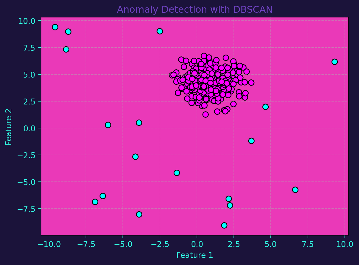
Density-Based Spatial Clustering of Applications with Noise (DBSCAN) emerges as a robust algorithm for anomaly detection. Unlike traditional methods, DBSCAN doesn’t assume a specific shape for clusters and can effectively isolate points in low-density regions as outliers.
Visualizing anomalies is crucial for interpreting model results. Scatter plots with DBSCAN labels provide an intuitive representation of the identified anomalies in the dataset.
Evaluating anomaly detection models poses challenges due to the scarcity of anomalies. Metrics such as precision, recall, and F1 score provide a nuanced understanding of the model’s performance.
from sklearn.metrics import precision_score, recall_score, f1_score
from sklearn.cluster import DBSCAN
from sklearn.datasets import make_blobs
import numpy as np
import matplotlib.pyplot as plt

# Function to generate a synthetic dataset with outliers
def generate_dataset_with_outliers(seed=42):
    np.random.seed(seed)
    X, _ = make_blobs(n_samples=300, centers=1, cluster_std=1, random_state=0)
    outliers = np.random.uniform(low=-10, high=10, size=(20, 2))
    return np.concatenate([X, outliers]), np.concatenate([np.zeros(300), -np.ones(20)])

# Step 1: Generate a synthetic dataset with outliers
X, y_true = generate_dataset_with_outliers()

# Step 2: Train a DBSCAN model for anomaly detection
dbscan = DBSCAN(eps=1, min_samples=5)
predicted_labels = dbscan.fit_predict(X)

# Step 3: Visualize anomalies with DBSCAN labels
fig, ax = plt.subplots()
scatter = ax.scatter(X[:, 0], X[:, 1], c=predicted_labels, cmap=plt.cm.cool, edgecolor='black', s=50)
ax.set_title('Anomaly Detection with DBSCAN', color=purple)
ax.set_xlabel('Feature 1', color=blue)
ax.set_ylabel('Feature 2', color=blue)
ax.grid(True, linestyle='--', alpha=0.5)
ax.tick_params(axis='x', colors=blue)
ax.tick_params(axis='y', colors=blue)
ax.set_facecolor(pink)
fig.set_facecolor(background)
plt.show()

# Step 4: Evaluate the model using precision, recall, and F1 score
precision = precision_score(y_true, predicted_labels, pos_label=-1)
recall = recall_score(y_true, predicted_labels, pos_label=-1)
f1 = f1_score(y_true, predicted_labels, pos_label=-1)

print(f"Precision: {precision:.2f}")
print(f"Recall: {recall:.2f}")
print(f"F1 Score: {f1:.2f}")
Precision: 1.00
Recall: 0.90
F1 Score: 0.95
Anomaly detection, powered by algorithms like DBSCAN, plays a vital role in uncovering irregularities in data. The combination of effective visualizations and evaluation metrics enables us to gain insights into the anomalies present, providing a foundation for critical decision-making in various domains.